Square inclusion, basic scheme
Description of the problem
In this tutorial, we will compute the effective elastic properties of a simple 2D microstructure in plane strain. More precisely, we consider a periodic microstructure made of a square inclusion of size \(a\), embedded in a unit-cell of size \(L\) (see Fig. 1).

Fig. 1 The periodic microstructure under consideration.
\(\mu_\mathrm i\) (resp. \(\mu_\mathrm m\)) denotes the shear modulus of the inclusion (resp. the matrix); \(\nu_\mathrm i\) (resp. \(\nu_\mathrm m\)) denotes the Poisson ratio of the inclusion (resp. the matrix).
The effective properties of this periodic microstructure are derived from the solution to the so-called corrector problem
where \(\mathbf u\) denotes the unknown, periodic displacement, \(\boldsymbol\varepsilon\) (resp. \(\boldsymbol\sigma\)) is the local strain (resp. stress) and \(\mathbf C\) is the local stiffness (inclusion or matrix). From the solution to the above problem, the effective stiffness \(\mathbf C^\mathrm{eff}\) is defined as the tensor mapping the macroscopic (imposed) strain \(\mathbf E=\langle\boldsymbol\varepsilon\rangle\) to the macroscopic stress \(\boldsymbol\sigma=\langle\boldsymbol\sigma\rangle\) (where quantities between angle brackets denote volume averages)
Note
This example is illustrated in two dimensions (\(d=2\)). However, it is implemented so as to be dimension independent, so that \(d=3\) should work out of the box.
In the present tutorial, we shall concentrate on the 1212 component of the effective stiffness, that is to say that the following macroscopic strain will be imposed
and the volume average \(\langle\sigma_{12}\rangle\) will be evaluated. To do so, the boundary value problem (1) is transformed into an integral equation, known as the Lippmann–Schwinger equation (Korringa, 1973; Zeller & Dederichs, 1973 ; Kröner, 1974) . This equation reads
where \(\mathbf C_0\) denotes the stiffness of the reference material, \(\boldsymbol\Gamma_0\) the related Green operator for strains, and \(\boldsymbol\varepsilon\) the local strain tensor. We will assume that the reference material is isotropic, with shear modulus \(\mu_0\) and Poisson ratio \(\nu_0\).
Following Moulinec and Suquet (1998), the above Lippmann–Schwinger equation (3) is solved by means of fixed point iterations
Finally, the above iterative scheme is discretized over a regular grid, leading to the basic uniform grid, periodic Lippmann–Schwinger solver.
Implementation of the Lippmann–Schwinger operator
We will call the operator
the Lippmann–Schwinger operator. In the present section, we show how this operator is implemented as a class with Janus. This will be done by composing two successive operators, namely (i) the local operator
where \(\boldsymbol\tau\) denotes the stress-polarization, and (ii) the Green operator for strains
For the implementation of the local operator defined by Eq. (5), it is first observed that \(\mathbf C_0\), \(\mathbf C_\mathrm{i}\) and \(\mathbf C_\mathrm{m}\) being isotropic materials, \(\mathbf C-\mathbf C_0\) is an isotropic tensor at any point of the unit-cell. In other words, both \(\mathbf C_\mathrm i-\mathbf C_0\) and \(\mathbf C_\mathrm m-\mathbf C_0\) will be defined as instances of FourthRankIsotropicTensor.
Furthermore, this operator is local. In other words, the output value in cell (i0, i1) depends on the input value in the same cell only (the neighboring cells are ignored). More precisely, we assume that a uniform grid of shape (n, n) is used to discretized Eq. (4). Then the material properties are constant in each cell, and we define delta_C[i0, i1, :, :] the matrix representation of \(\mathbf C-\mathbf C_0\) (see Mandel notation). Likewise, eps[i0, i1, :] is the vector representation of the strain tensor in cell (i0, i1). Then, the stress-polarization \(\left(\mathbf C-\mathbf C_0\right):\boldsymbol\varepsilon\) in cell (i0, i1) is given by the expression:
tau[i0, i1] = delta_C[i0, i1] @ eps[i0, i1],
where @ denotes the matrix multiplication operator. It results from the above relation that the lcoal operator defined by (5) should be implemented as a BlockDiagonalOperator2D. As for the non-local operator, it is instanciated by a simple call to the green_operator method of the relevant material (see Materials).
The script starts with imports from the standard library, the SciPy stack and Janus itself:
import itertools

import numpy as np
import matplotlib.pyplot as plt

import janus.green as green
import janus.fft.serial as fft
import janus.material.elastic.linear.isotropic as material
import janus.operators as operators

from janus.operators import isotropic_4
We then define a class Example, which represents the microsctructure described above. The first few lines of its initializer are pretty simple
class Example:
    def __init__(self, mat_i, mat_m, mat_0, n, a=0.5, dim=3):
        self.mat_i = mat_i
        self.mat_m = mat_m
        self.n = n
        shape = tuple(itertools.repeat(n, dim))
        # ...
mat_i (resp. mat_m, mat_0) are the material properties of the inclusion (resp. the matrix, the reference material); n is the number of grid cells along each side, a is the size of the inclusion, and dim is the dimension of the physical space. The shape of the grid is stored in a tuple, the length of which depends on dim.
Note
As much as possible, keep your code dimension-independent. This means that the spatial dimension (2 or 3) should not be hard-coded. Rather, you should make it a rule to always parameterize the spatial dimension (use a variable dim), even if you do not really intend to change this dimension. Janus object sometimes have different implementations depending on the spatial dimension. For example, the abstract class FourthRankIsotropicTensor has two concrete daughter classes FourthRankIsotropicTensor2D and FourthRankIsotropicTensor3D. However, both can be instantiated through the unique function isotropic_4, where the spatial dimension can be specified.
We then define the local operators \(\mathbf C_\mathrm i-\mathbf C_0\) and \(\mathbf C_\mathrm m-\mathbf C_0\) as FourthRankIsotropicTensor. It is recalled that the stiffness \(\mathbf C\) of a material with bulk modulus \(\kappa\) and shear modulus \(\mu\) reads
where \(d\) denotes the dimension of the physical space and \(\mathbf J\) (resp. \(\mathbf K\)) denote the spherical (resp. deviatoric) projector tensor. In other words, the spherical and deviatoric projections of \(\mathbf C\) are \(d\kappa\) and \(2\mu\), respectively. As a consequence, the spherical and deviatoric projections of \(\mathbf C-\mathbf C_0\) are \(d\left(\kappa-\kappa_0\right)\) and \(2\left(\mu-\mu_0\right)\), respectively. This leads to the following definitions
        # ...
        delta_C_i = isotropic_4(dim*(mat_i.k-mat_0.k),
                                2*(mat_i.g-mat_0.g), dim)
        delta_C_m = isotropic_4(dim*(mat_m.k-mat_0.k),
                                2*(mat_m.g-mat_0.g), dim)
        # ...
Now, delta_C_i and delta_C_m are used to create the operator \(\boldsymbol\varepsilon\mapsto\left(\mathbf C-\mathbf C_0\right):\boldsymbol\varepsilon\) as a BlockDiagonalOperator2D. Block-diagonal operators are initialized from an array of local operators, called ops below
Todo
This code snippet is not dimension independent.
        # ...
        ops = np.empty(shape, dtype=object)
        ops[:, :] = delta_C_m
        imax = int(np.ceil(n*a-0.5))
        ops[:imax, :imax] = delta_C_i
        self.eps_to_tau = operators.BlockDiagonalOperator2D(ops)
        # ...
The upper-left quarter of the unit-cell is filled with delta_C_i (\(\mathbf C_\mathrm i-\mathbf C_0\)), while the remainder of the unit-cell receives delta_C_m (\(\mathbf C_\mathrm m-\mathbf C_0\)). Finally, a BlockDiagonalOperator2D is created from the array of local operators. It is called eps_to_tau as it maps the strain (\(\boldsymbol\varepsilon\)) to the stress-polarization (\(\boldsymbol\tau\)).
Note
eps_to_tau is not a method. Rather, it is an attribute, which turns out to be a function.
Finally, the discrete Green operator for strains associated with the reference material \(\mathbf C_0\) is created. This requires first to create a FFT object (see Computing discrete Fourier transforms).
Todo
Document Green operators for strains.
        # ...
        self.green = green.truncated(mat_0.green_operator(),
                                     shape, 1.,
                                     fft.create_real(shape))
The Lippmann–Schwinger operator \(\boldsymbol\varepsilon\mapsto\boldsymbol\Gamma_0[\left(\mathbf C-\mathbf C_0\right):\boldsymbol\varepsilon]\) is then defined by composition
    def apply(self, x, out=None):
        if out is None:
            out = np.zeros_like(x)
        self.eps_to_tau.apply(x, out)
        self.green.apply(out, out)
which closes the definition of the class Example.
Note
Note how we allowed for the output array to be passed by reference, thus allowing for memory reuse.
The main block of the script
It starts with the definition of a few parameters
if __name__ == '__main__':
    dim = 2                # Spatial dimension
    sym = (dim*(dim+1))//2 # Dim. of space of second rank, symmetric tensors
    n = 256                # Number of cells along each side of the grid
    mu_i, nu_i = 100, 0.2  # Shear modulus and Poisson ratio of inclusion
    mu_m, nu_m = 1, 0.3    # Shear modulus and Poisson ratio of matrix
    mu_0, nu_0 = 50, 0.3   # Shear modulus and Poisson ratio of ref. mat.
    num_cells = n**dim     # Total number of cells
Then, an instance of class Example is created
    example = Example(mat_i=material.create(mu_i, nu_i, dim),
                      mat_m=material.create(mu_m, nu_m, dim),
                      mat_0=material.create(mu_0, nu_0, dim),
                      n=n,
                      dim=dim)
We then define eps_macro, which stores the imposed value of the macroscopic strain \(\mathbf E\), and eps and eps_new, which hold two successive iterates of the local strain field \(\boldsymbol\varepsilon\).
    avg_eps = np.zeros((sym,), dtype=np.float64)
    avg_eps[-1] = 1.0

    eps = np.empty(example.green.ishape, dtype=np.float64)
    new_eps = np.empty_like(eps)
Note
The shape of the arrays eps and eps_new is simply inferred from the shape of the input of the Green operator for strains \(\boldsymbol\Gamma_0\).
We will not implement a stopping criterion for this simple example. Rather, a fixed number of iterations will be specified. Meanwhile, the residual
will be computed and stored at each iteration through the following estimate
norm(new_eps-eps)/sqrt(num_cells)/norm(avg_eps),
where normalization (using \(\lVert\mathbf E\rVert\)) is also applied.
Note
Note that the quantity defined by Eq. (7) is truly a residual. Indeed, it is the norm of the difference between the left- and right-hand side in Eq. (3), since \(\boldsymbol\varepsilon^{k+1}-\boldsymbol\varepsilon^k=\mathbf E-\boldsymbol\Gamma_0[\left(\mathbf C-\mathbf C_0\right):\boldsymbol\varepsilon^k]-\boldsymbol\varepsilon^k\).
The fixed-point iterations defined by Eq. (4) are then implemented as follows
    num_iter = 400
    res = np.empty((num_iter,), dtype=np.float64)
    eps[...] = avg_eps
    normalization = 1/np.sqrt(num_cells)/np.linalg.norm(avg_eps)

    for i in range(num_iter):
        example.apply(eps, out=new_eps)
        np.subtract(avg_eps, new_eps, out=new_eps)
        res[i] = normalization*np.linalg.norm(new_eps-eps)
        eps, new_eps = new_eps, eps
and the results are post-processed
    tau = example.eps_to_tau.apply(eps)
    avg_tau = np.mean(tau, axis=tuple(range(dim)))
    C_1212 = mu_0+0.5*avg_tau[-1]/avg_eps[-1]
    print(C_1212)

    fig, ax = plt.subplots()
    ax.set_xlabel('Number of iterations')
    ax.set_ylabel('Normalized residual')
    ax.loglog(res)
    fig.tight_layout(pad=0.2)
    fig.savefig('residual.png', transparent=True)

    fig, ax_array = plt.subplots(nrows=1, ncols=3)
    width, height = fig.get_size_inches()
    fig.set_size_inches(width, width/3)
    for i, ax in enumerate(ax_array):
        ax.set_axis_off()
        ax.imshow(eps[..., i], interpolation='nearest')
    fig.tight_layout(pad=0)
    fig.savefig('eps.png', transparent=True)
To compute the macroscopic stiffness, we recall the definition of the stress-polarization from which we find
Then, from the specific macroscopic strain \(\mathbf E\) that we considered [see Eq. (2)]
where brackets refer to the Mandel notation, and the -1 index denotes the last component of the column-vector (which, in Mandel’s notation, refers to the 12 component of second-rank symmetric tensors, both in two and three dimensions). We get the following approximation
C_1212 # 1.41903971282,
and the map of the local strains is shown in Fig. 2, while Fig. 3 shows that the residual decreases (albeit slowly) with the number of iterations. This completes this tutorial.
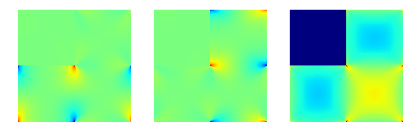
Fig. 2 The maps of \(\boldsymbol\varepsilon_{11}\) (left), \(\boldsymbol\varepsilon_{22}\) (middle) and \(\boldsymbol\varepsilon_{12}\) (right). Different color scales were used for the left and middle map, and for the right map. Note that in the above representation, the \(x_1\) axis points to the bottom, while the \(x_2\) axis points to the right.
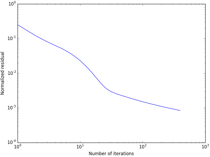
Fig. 3 The normalized residual as a function of the number of iterations.
The complete program
The complete program can be downloaded here.
# Begin: imports
import itertools

import numpy as np
import matplotlib.pyplot as plt

import janus.green as green
import janus.fft.serial as fft
import janus.material.elastic.linear.isotropic as material
import janus.operators as operators

from janus.operators import isotropic_4
# End: imports

# Begin: init
class Example:
    def __init__(self, mat_i, mat_m, mat_0, n, a=0.5, dim=3):
        self.mat_i = mat_i
        self.mat_m = mat_m
        self.n = n
        shape = tuple(itertools.repeat(n, dim))
        # ...
        # End: init
        # Begin: create (C_i - C_0) and (C_m - C_0)
        # ...
        delta_C_i = isotropic_4(dim*(mat_i.k-mat_0.k),
                                2*(mat_i.g-mat_0.g), dim)
        delta_C_m = isotropic_4(dim*(mat_m.k-mat_0.k),
                                2*(mat_m.g-mat_0.g), dim)
        # ...
        # End: create (C_i - C_0) and (C_m - C_0)
        # Begin: create local operator ε ↦ (C-C_0):ε
        # ...
        ops = np.empty(shape, dtype=object)
        ops[:, :] = delta_C_m
        imax = int(np.ceil(n*a-0.5))
        ops[:imax, :imax] = delta_C_i
        self.eps_to_tau = operators.BlockDiagonalOperator2D(ops)
        # ...
        # End: create local operator ε ↦ (C-C_0):ε
        # Begin: create non-local operator ε ↦ Γ_0[ε]
        # ...
        self.green = green.truncated(mat_0.green_operator(),
                                     shape, 1.,
                                     fft.create_real(shape))
        # End: create non-local operator ε ↦ Γ_0[ε]


    # Begin: apply
    def apply(self, x, out=None):
        if out is None:
            out = np.zeros_like(x)
        self.eps_to_tau.apply(x, out)
        self.green.apply(out, out)
    # End: apply


# Begin: params
if __name__ == '__main__':
    dim = 2                # Spatial dimension
    sym = (dim*(dim+1))//2 # Dim. of space of second rank, symmetric tensors
    n = 256                # Number of cells along each side of the grid
    mu_i, nu_i = 100, 0.2  # Shear modulus and Poisson ratio of inclusion
    mu_m, nu_m = 1, 0.3    # Shear modulus and Poisson ratio of matrix
    mu_0, nu_0 = 50, 0.3   # Shear modulus and Poisson ratio of ref. mat.
    num_cells = n**dim     # Total number of cells
    # End: params
    # Begin: instantiate example
    example = Example(mat_i=material.create(mu_i, nu_i, dim),
                      mat_m=material.create(mu_m, nu_m, dim),
                      mat_0=material.create(mu_0, nu_0, dim),
                      n=n,
                      dim=dim)
    # End: instantiate example
    # Begin: define strains
    avg_eps = np.zeros((sym,), dtype=np.float64)
    avg_eps[-1] = 1.0

    eps = np.empty(example.green.ishape, dtype=np.float64)
    new_eps = np.empty_like(eps)
    # End: define strains
    # Begin: iterate
    num_iter = 400
    res = np.empty((num_iter,), dtype=np.float64)
    eps[...] = avg_eps
    normalization = 1/np.sqrt(num_cells)/np.linalg.norm(avg_eps)

    for i in range(num_iter):
        example.apply(eps, out=new_eps)
        np.subtract(avg_eps, new_eps, out=new_eps)
        res[i] = normalization*np.linalg.norm(new_eps-eps)
        eps, new_eps = new_eps, eps
    # End: iterate
    # Begin: post-process
    tau = example.eps_to_tau.apply(eps)
    avg_tau = np.mean(tau, axis=tuple(range(dim)))
    C_1212 = mu_0+0.5*avg_tau[-1]/avg_eps[-1]
    print(C_1212)

    fig, ax = plt.subplots()
    ax.set_xlabel('Number of iterations')
    ax.set_ylabel('Normalized residual')
    ax.loglog(res)
    fig.tight_layout(pad=0.2)
    fig.savefig('residual.png', transparent=True)

    fig, ax_array = plt.subplots(nrows=1, ncols=3)
    width, height = fig.get_size_inches()
    fig.set_size_inches(width, width/3)
    for i, ax in enumerate(ax_array):
        ax.set_axis_off()
        ax.imshow(eps[..., i], interpolation='nearest')
    fig.tight_layout(pad=0)
    fig.savefig('eps.png', transparent=True)
    # End: post-process