What is homogenization? Part 3: ensemble averages vs. volume averages

In the previous instalment of this series on homogenization, we discussed homogenization of a distribution of black dots on a white background to a uniform shade of gray. In that example, homogenization boils down to evaluating the fraction of the total area occupied by the dots: this is the so-called rule of mixtures. Of course, in most real-case applications, the homogenization process is much more complex than merely evaluating a surface (or volume) fraction. However, before we move onto such more difficult homogenization processes, we will discuss in more detail volume fractions in the present post, where we will introduce periodic and random homogenization.

In the halftoning example that we used previously, computing the effective gray-level was fairly easy owing to the fact that the dots were regularly spaced. The pattern is in fact periodic: the whole plane (or space) can be paved with one single unit-cell (a hexagon in the present case).

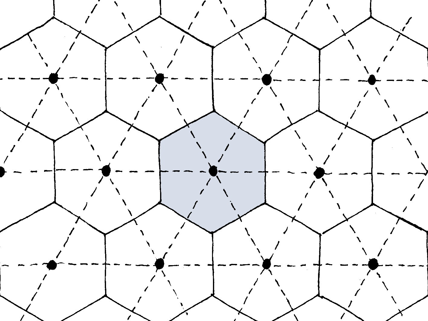
Once the unit-cell had been identified, the effective gray-level was computed as the following surface fraction

$$\text{effective gray level} = \frac{\text{surface area of white region}}{\text{surface area of unit-cell}}.$$

This is an example of what is called periodic homogenization, meaning that the heterogeneities are laid out in a periodic pattern. Homogenization in the periodic case is generally a three-step process:

1. identify the unit-cell,
2. solve an auxiliary problem on the unit-cell,
3. post-process the solution to the auxiliary problem to compute the effective properties.

In the above example:

1. the unit-cell is a hexagon,
2. the auxiliary problem reads: “compute the surface area of the unit-cell and the surface area of the white region”,
3. post-processing reduces to forming the surface ratio.

In reality, most natural and manufactured materials are not as regular as the pattern considered above. They are in fact disordered. For example, the distribution of holes (pores) in the following (manufactured) sponge does not follow a regular pattern.

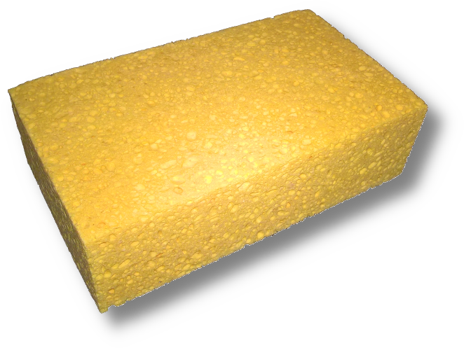
So, how do we move from the simple, periodic case to the more realistic, disordered case? The keyword is: “random process”. We assume that the material at hand is the result of a random process. I must insist, here: this is an assumption, and wording does matter. What we truly have is a disordered material (meaning that it's all very messy in here). Representing this disordered material as the result of a random process is a modelling assumption. It implies some kind of reproducibility, in the sense that the same random process can be reproduced many times, each time resulting in what we will call a new realization of essentially the same disordered material. The realizations are indeed different, but (very losely speaking) they carry the “same kind of randomness” (they look similar). The important consequence of this assumption is that it is possible to describe the disordered material statistically. This is illustrated below with the sponge shown previously.

In the case of the sponge, reproducibility is in fact a highly desirable feature, since the manufacturer wants to insure the quality of his product remains constant. To do so, he keeps the conditions (raw materials, temperature, relative humidity, …) identical. Describing the sponge as a random process is extremely natural in that case.

It is time to formalize the above discussion. To do so, we rely on the sponge and make the simplifying assumption that the solid (yellow) phase is homogeneous. Then, the disordered material is fully described by the indicator function $\chi(\vec x)$ of the solid phase: $\chi(\vec x)=1$ if $\vec x$ belongs to the solid phase, $\chi(\vec x)=0$ otherwise. Of course, the indicator function $\chi$ is different for each new realization. This is acknowleged by the introduction of a second argument to the function $\chi$, namely: $\omega.$ This argument is formal, it refers to the realization (see also the Wikipedia page on random variables). To sum up: the microstructure of the sponge is defined by the function $\chi(\vec x, \omega)$, where $\vec x$ is the observation point and $\omega$ is the realization. By freezing each of these two parameters in turn, we will define two kinds of averages of $\chi$.

Let us assume that you pay a visit to the sponge manufacturer and get permission to look at all sponges that were produced this day. For each of these sponges, you carry out the following experiment: “observe the content (solid or void) at a fixed point (say, the center of the top face)”. In other words, for fixed $\vec x$, you measure $\chi(\vec x, \omega_1), \ldots, \chi(\vec x, \omega_N)$, where $\omega_1,\ldots, \omega_N$ denote the sponges under scrutiny. The empirical probability that point $\vec x$ belongs to the solid phase is

$$P[\chi(\vec x, \omega)=1]=\frac1N\sum_{i=1}^N\chi(\vec x, \omega_i).$$

The above probability can also be seen as the expectation of $\chi(\vec x, \omega)$, for fixed observation point $\vec x$

$$\mathbb{E}(\chi)(\vec x)=0\times P[\chi(\vec x, \omega)=0]+1\times P[\chi(\vec x, \omega)=1],$$

and it results from the above discussion that $\mathbb E(\chi)(\vec x)$ is the “frequency of occurence” of the solid phase at point $\vec x$. Note that this ensemble average depends in theory on the observation point $\vec x$. However, we will only consider in the present series random materials that are statistically homogeneous. For such materials $\mathbb E(\chi)(\vec x)$ is a constant that does not depend on the observation point¹. Homogeneity is an important property: it means that, statistically speaking, all points are equivalent (they carry the “same randomness”). For statistically homogeneous materials, we will write $\mathbb E(\chi)$ rather than $\mathbb E(\chi)(\vec x)$, since the observation point $\vec x$ is irrelevant.

The ensemble average $\mathbb E(\chi)$ was obtained above by freezing the first variable $\vec x$ in $\chi(\vec x, \omega)$. We now freeze the second variable, $\omega.$ Let us assume that, before taking leave from the manufacturer, you took one sponge with you. Back home from the sponge factory, you decide to observe the sponge at $N$ points $\vec x_1, \ldots, \vec x_N$. These points are regularly spaced on a 3D grid. In other words, you measure $\chi(\vec x_i, \omega)$ for $i=1, \ldots, N$ ($N$ is now the number of points, not the number of samples). The following average

$$\frac 1N\sum_{i=1}^N\chi(\vec x_i, \omega)$$

is an estimate of the fraction of points that are located in the solid phase. In the limit of very dense 3D grids, the above sum converges to an integral

$$\frac 1N\sum_{i=1}^N\chi(\vec x_i, \omega)\to\frac 1V\int_{\Omega}\chi(\vec x, \omega)\,\D V,$$

where $\Omega$ denotes the domain occupied by the sponge, and $V$ its volume. This quantity is the volume average $\langle\chi\rangle(\omega)$ of $\chi$

$$\langle\chi\rangle(\omega)=\frac1V\int_{\Omega}\chi(\vec x, \omega)\,\D V.$$

The volume average depends on the realization $\omega$: in other words, the volume fraction of solid may vary from one sponge to another. However, we do know intuitively that for sufficiently large sponges, the volume average will in fact not depend on the realization. This property is not universal, though. It characterizes so-called ergodic materials. Very roughly speaking, for ergodic materials, volume averages over large domains converge to the ensemble average

$$\lim_{V\to+\infty}\frac1V\int_{\Omega}\chi(\vec x, \omega)\,\D V\to\mathbb E(\chi).$$

This limit is sometimes called the thermodynamic limit. It will always be assumed in this series that the materials considered are ergodic.

Conclusion

This post was a small detour on our way to homogenization. We previously introduced homogenization of a periodic microstructure, while what we really would like to define is homogenization of disordered microstructures. Modelling such disordered microstructures as random processes, we were able to define two kinds of averages of a quantity: the ensemble average over the realizations (the observation point being fixed) and the volume average over the domain (the realization being fixed). For statistically homogeneous materials, the ensemble average does not depend on the observation point. Furthermore, for ergodic materials, the volume average over a large domain coincides with the ensemble average.

In the next post, we will consider our first homogenization example.