Orientation correlations among rice grains, part 6: segmentation

In the previous instalment of this series, I showed that a convincing binary image could be produced from the gray level 3D reconstruction of the assembly of rice grains, using Otsu's threshold. However, I intend to carry out statistical analyses of the grains themselves in the subsequent instalments. Therefore, instead of a binary image of the rice grains, what is really needed is a labelled image, where all voxels which are thought to belong to the same rice grain are tagged with the same label. This is called segmentation, which is the topic of the present post. I will first show that the most basic segmentation technique (namely, detecting connected components in the image) fails in the present case. This calls for a more elaborate strategy, based on the widely popular watershed method. However, blind application of the standard watershed strategy leads to over-segmentation. This post will therefore close on a problem-dependent strategy better suited to the present case.

Before we start, let me mention a book-keeping issue. Up to the previous post, 2D slices of the 3D image were stored in separate *.tif files, which is rather tedious to load and solve. From now on, I will store all analyses in a *.hdf5 file. I am by no means an expert on this great file format (see website), but what I like about it is

1. it is language-agnostic,
2. it is platform- (and architecture-) independent: no indianness problem,
3. several arrays can be stored in the same file,
4. comments can be attached to a dataset.

The following code snippet (download) converts the binary *.tif images into a single *.hdf5 file. It uses the h5py library; PyTables is another option.

import os.path

import h5py
import numpy as np
import skimage.io

if __name__ == '__main__':
    root =  os.path.join('F:\\', 'sebastien', 'experimental_data', 'navier',
                         'riz')
    input_name = os.path.join(root, 'bin_4x4x4-otsu',
                              'rice-bin_4x4x4-otsu_126-{0:03d}.tif')
    output_name = os.path.join(root, 'rice-bin_4x4x4.hdf5')
    num_slices = 172

    binary = None
    for i in range(num_slices):
        slc = skimage.io.imread(input_name.format(i))
        if binary is None:
            binary = np.zeros((num_slices,)+slc.shape, dtype=slc.dtype)
        binary[i] = slc

    with h5py.File(output_name, 'w') as f:
        dset=f.create_dataset('binary', data=binary)
        dset.attrs['description'] = np.string_('Otsu threshold 126')

Now, on to segmentation!

Detecting connected components

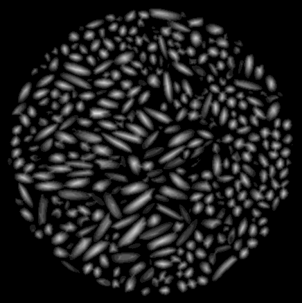
This is probably the most simple segmentation technique. In this approach, a feature is defined as a connected component of the image. Let's be honnest: it rarely works on real-life images, because most of the times, distinct objects usually touch, and therefore appear as connected. Fig. 1 shows that our 3D image is no exception to this rule!

So, we should expect no miracle from this approach. However, it is interesting to show how easy it is to identify the connected components of an image, using the scipy.ndimage module (documentation), in particular the scipy.ndimage.label function (documentation). Note the use of np.ones((3, 3, 3)) as a structuring element, meaning 26-connectivity.

import os.path

import h5py
import numpy as np

from scipy import ndimage as ndi
from skimage.io import imsave

if __name__ == '__main__':
    root =  os.path.join('F:\\', 'sebastien', 'experimental_data', 'navier',
                         'riz')
    with h5py.File(os.path.join(root, 'rice-bin_4x4x4.hdf5')) as f:
        binary = np.asarray(f['binary'])

    print('Selecting markers from distance local maxima...')
    labels, num_labels = ndi.label(binary,
                                   structure=np.ones((3, 3, 3), dtype=np.int8))
    print('    ... found {} connected components'.format(num_labels))

    index = 100
    np.random.seed(20150928)
    colors = np.random.randint(255, size=(labels.max()+1, 3)).astype(np.uint8)
    colors[0] = [0, 0, 0]

    imsave('connected_components.png', colors[labels[index]])

The above code snippet (download) detects 117 connected components, and produces the following colored image (one color per label), see Fig. 2. Unsurprisingly, all grains are connected on this slice, and we have produced a very poor segmentation indeed!

To close this section, it should be noted that the last lines of the above script produce a color image where each label receives a random color. Standard color maps are indeed ill-suited to visualization of labelled images. Indeed, these color maps are most of the times smooth, which means that close labels are barely distinguishable. This is undesirable, since neighbouring features usually get close labels.

Also note the use of advanced indexing of the Numpy arrays (colors[labels[index]])... Python and Numpy rock!

Watershed segmentation, blind application

The watershed segmentation is a very popular technique to segment overlapping objects. Describing this technique is out of the scope of this post. Suffice it to say that watershed segmentation is a three-step process

1. compute the topography of the image (usually, a gradient map or the opposite of the distance map to the background),
2. select seeds,
3. grow connected region from seeds.

The second step is the critical one, since each seed results in exactly one feature in the segmented image. Too many seeds result in an oversegmented image (grains are split), while too little seeds result in an under-segmented image (grains are merged).

While tedious, manual seeding is probably your best choice (as argued by Emmanuelle Gouillart). There are about 2000 rice grains in the 3D image we are working with, so this semi-supervised approach is unfortunately not an option for us.

The standard unsupervised seeding technique consists in selecting the local maxima of the map of the distance to the background. The opposite of the distance map is then used as topography. This is essentially what the script below does (download). It draws heavily on the example from the scikit-image documentation.

"""Watershed using local maxima of the distance map as seeds."""

import os.path

import h5py
import numpy as np

from scipy import ndimage as ndi
from skimage.feature import peak_local_max
from skimage.io import imread, imsave, imshow
from skimage.morphology import watershed

def markers_from_distance_local_max(image, distance=None, min_distance=10):
    if distance is None:
        distance = ndi.distance_transform_edt(image)
    return

if __name__ == '__main__':
    root =  os.path.join('F:\\', 'sebastien', 'experimental_data', 'navier',
                         'riz')
    with h5py.File(os.path.join(root, 'rice-bin_4x4x4.hdf5')) as f:
        binary = np.asarray(f['binary'])

    print('Computing distance transform')
    distance = ndi.distance_transform_edt(binary)

    print('Selecting markers from distance local maxima...')
    local_maxi = peak_local_max(distance, labels=binary,
                                min_distance=10,
                                indices=False)
    markers, num_seeds = ndi.label(local_maxi,
                                   structure=np.ones((3, 3, 3), dtype=np.int8))
    print('    ... found {} seeds'.format(num_seeds))

    print('Computing watershed transform')
    labels = watershed(-distance, markers, mask=binary)

    index = 100
    np.random.seed(20150929)
    colors = np.random.randint(255, size=(labels.max()+1, 3)).astype(np.uint8)
    colors[0] = [0, 0, 0]

    imsave('distance.png', distance[index]/distance.max())
    imsave('watershed-distance_local_max.png', colors[labels[index]])

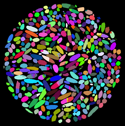
The result of this operation is shown on Fig. 3, where over-segmentation is observed. The reason for this is very simple, and typical of elongated objects: there are several local maxima of the distance map in each grain (see Fig. 4), resulting in too many seeds.

One possible response would be to use so-called vertical filters (Tariel et al., 2008). I used here a more intuitive approach by providing a min_distance parameter to the scikit-image peak_local_max (documentation) function. The selected value (namely, 10 px) corresponds to the typical equatorial radius of the rice grains (as manually measured on the binary images). This indeed reduces over-segmentation, but does not solve the problem completely.

In the next section, we will see how a problem dependent solution can be proposed.

Watershed segmentation with directional erosion

In the previous section, over-segmentation occured because of the anisotropy of the objects. In other words, had the grains been nearly spherical, then we would have produced a very convincing segmentation with the above method.

The grains are elongated: this is a fact. Instead of ignoring it (at the cost of over-segmentation), we should take this important piece of information into account in the seeding process. In the present section I propose to erode the binary image with elongated structuring elements. Only those grains which have roughly the same orientation as the structuring element will remain. If we vary the orientation of the structuring element, we should be able to seed each grain.

The proposed procedure is summarized below.

1. Generate a set of orientations: we will use the vertices of an icosahedron, which give 20 orientations, uniformly distributed on the unit sphere.
2. Generate the corresponding ellipsoidal structuring elements, using the class Spheroid, defined here. I will not comment this module in the present post (I might make it the topic of a future post!). Suffice it to say that the aspect ratio of the structuring element is close to that of the actual rice grains. The structuring element should be neither too small, nor too large. I (manually) selected an equatorial radius of 3.5 px, and a polar radius of 9.5 px.
3. Generate 20 eroded images.
4. Evaluate the OR combination of the 20 eroded images.
5. Identify the connected components of the combined eroded images.
6. Use these connected components to seed the watershed process.

The resulting script is very simple (download).

"""Watershed using directional erosions."""

import os.path

import h5py
import numpy as np

from scipy import ndimage as ndi
from skimage.feature import peak_local_max
from skimage.io import imread, imsave, imshow
from skimage.morphology import watershed

from spheroid import Spheroid


def icosahedron():
    t = (1+np.sqrt(5))/2
    u = t/np.sqrt(1+t**2)
    v = 1/np.sqrt(1+t**2)
    vertices = np.array([[ u,  v,  0], [-u,  v,  0], [ u, -v,  0],
                         [-u, -v,  0], [ v,  0,  u], [ v,  0, -u],
                         [-v,  0,  u], [-v,  0, -u], [ 0,  u,  v],
                         [ 0, -u,  v], [ 0,  u, -v], [ 0, -u, -v]],
                        dtype=np.float64)
    faces = np.array([[ 0,  8,  4], [ 0,  5, 10], [ 2,  4,  9], [ 2, 11,  5],
                      [ 1,  6,  8], [ 1, 10,  7], [ 3,  9,  6], [ 3,  7, 11],
                      [ 0, 10,  8], [ 1,  8, 10], [ 2,  9, 11], [ 3, 11,  9],
                      [ 4,  2,  0], [ 5,  0,  2], [ 6,  1,  3], [ 7,  3,  1],
                      [ 8,  6,  4], [ 9,  4,  6], [10,  5,  7], [11,  7,  5]],
                     dtype=np.uint8)
    return vertices, faces


if __name__ == '__main__':
    root =  os.path.join('F:\\', 'sebastien', 'experimental_data', 'navier',
                         'riz')
    with h5py.File(os.path.join(root, 'rice-bin_4x4x4.hdf5')) as f:
        binary = np.asarray(f['binary'])

        print('Computing distance transform')
        distance = ndi.distance_transform_edt(binary)
        dset = f.create_dataset('distance', data=distance)
        dset.attrs['description'] = np.string_('distance transform of `binary`')

        print('Selecting markers from directional erosion...')
        a, c = 3.5, 9.5
        vertices  = icosahedron()[0]
        eroded = np.zeros_like(binary, dtype=np.bool)
        for v in vertices:
            spheroid = Spheroid(a, c, v).digitize()
            np.logical_or(eroded,
                          ndi.binary_erosion(binary,
                                             structure=spheroid),
                          out=eroded)
        markers, num_seeds =  ndi.label(eroded,
                                        structure=np.ones((3, 3, 3),
                                                          dtype=np.int8))
        dset = f.create_dataset('markers', data=markers)
        descr = ('`binary` image was eroded with 20 spheroids '+
                 '(a={}, c={}) '.format(a, c)+
                 'using the vertices of a icosahedron as orientations. This'+
                 'image is the logical OR of all 20 eroded images.')
        dset.attrs['description'] = np.string_(descr)
        print('    ... found {} seeds'.format(num_seeds))

        print('Computing watershed transform')
        labels = watershed(-distance, markers, mask=binary)
        dset = f.create_dataset('labels', data=labels)
        descr = 'watershed using `markers` and the opposite of `distance`.'
        dset.attrs['description'] = np.string_(descr)

    index = 100
    np.random.seed(20150924)
    colors = np.random.randint(255, size=(labels.max()+1, 3)).astype(np.uint8)
    colors[0] = [0, 0, 0]

    imsave('distance.png', distance[index]/distance.max())
    imsave('makers-directional_erosion.png', colors[markers[index]])
    imsave('watershed-directional_erosion.png', colors[labels[index]])

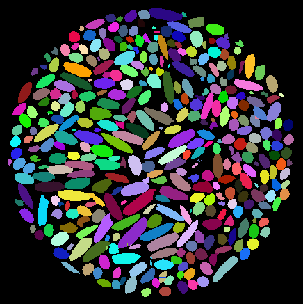
It identifies 2362 seeds (instead of 2672 in the previous approach). The resulting segmentation is shown in Fig. 5. It can be seen that we almost got rid of over-segmentation.

Conclusion

In an image analysis pipeline, segmentation is notoriously the critical step of the process. Watershed is a very efficient technique, which requires careful seeding. For anisotropic object, ad-hoc techniques have to be adopted. In the present blog, I showed how some simple mathematical morphology operations could be used to produce a satisfactory set of seeds. It should be noted however that the reason why the proposed approach works so well is that rice grains are nearly spheroidal. In other words, correctly seeding the watershed process is highly problem dependent!

In the next instalment of this series, I will show how to analyse the shape and orientation of each individual grain.