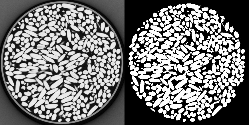
In the previous instalment of this series, we used the circle Hough transform to find the boundary of the sample and define the circular ROI. Within this ROI, we now need to segment the rice grains. In other words, starting from a gray-level image (Fig. 1, left), we want to produce a binary image, where all pixels that we believe belong to rice grains are white, and all background pixels are black (Fig. 1, right). This is the topic of the present post, where we will use Otsu's automated threshold selection. I will first discuss Otsu's method, and propose what I believe is a new interpretation of this rather old technique. Then, I will apply this method to the 3D image of rice grains, using scikit-image.

Plotting the image's histogram

Before we dig into Otsu's method, we will first draw the histogram of the original image shown in Fig. 1 (left), remembering that the boundary was found in the previous instalment to be a circle centered at (219, 217), with radius 208. The following Python code computes and saves the histogram as a SVG file, which is displayed in Fig. 2.

import os.path

import numpy as np
import matplotlib as mpl
import matplotlib.pyplot as plt

from skimage.draw import circle
from skimage.io import imread

root = "."

img = imread(os.path.join(root, "rice-bin_4x4x4-099.tif"))
rows, cols = circle(219, 217, 208)

mpl.style.use(os.path.join(root, "sb-blog.mplstyle"))
fig = mpl.figure.Figure(figsize=(8, 3))
ax = fig.add_subplot(1, 1, 1)
h, bins, patches = ax.hist(img[rows, cols], bins=256, range=(0, 256),
                           histtype='stepfilled',
                           color='b', alpha=0.5, linewidth=0)
ax.set_xlabel('Gray value')
ax.set_ylabel('Pixel count')
ax.set_xlim(0, 250)
ax.xaxis.set_minor_locator(mpl.ticker.AutoMinorLocator(5))
fig.tight_layout()
fig.savefig(os.path.join(root, 'rice-bin_4x4x4-hist-099.svg'),
            transparent=True)

/usr/lib/python3/dist-packages/matplotlib/tight_layout.py:231: UserWarning: tight_layout : falling back to Agg renderer
  warnings.warn("tight_layout : falling back to Agg renderer")

It is observed that this histogram is relatively well suited to thresholding. Indeed, it exhibits two peaks which are fairly well-separated, and the pixel counts between these peaks are rather small. However, these pixel counts never go to zero, which means that no matter the threshold, the thresholded image will always be wrong!

Otsu's method

Otsu's method (Otsu, 1979) is a popular thresholding technique. It is quite effective on simple images, when the histogram has two well separated peaks. Otsu\'s optimum threshold is often presented as (quoted from Wikipedia)

separating the two classes so that their combined spread (intra-class variance) is minimal, or equivalently (because the sum of pairwise squared distances is constant), so that their inter-class variance is maximal.

I have always found this definition non-intuitive. Why should maximizing the intra-class variance return a satisfactorily thresholded image? Well, I came to develop my own understanding of Otsu's method.

We start with the original (noisy) image, which will be considered as a map $f\colon E\to{0,\ldots,L-1}$ from the set $E$ of pixels to the set ${0,\ldots,L-1}$ of gray levels ($L$ denotes the total number of gray levels). It should be noted that in Otsu's original paper (1979), the gray levels span ${1,\ldots,L}$ rather than ${0,\ldots,L-1}$: the convention adopted here is more in line with standard images.

We want to find the “best” binary approximation of $f$, in the sense of Problem 1 defined below.

Problem 1: Find two gray levels $g_0$ and $g_1$, and the map $g\colon E\to{g_0, g_1}$ that minimizes the distance

$$d(f, g)^2=\sum_{x\in E}\left[f(x)-g(x)\right]^{2}.$$

At this point, it should be noted that the above choice of distance will result in $g$ being the maximum likelihood estimator of $f$ in the presence of Gaussian noise (a common assumption in image analysis – even if noise rather follows a Poisson distribution on real detectors). It can readily be verified that Problem 1 in fact reduces to Otsu's method! To prove this assertion, we need to rewrite this problem. Let $g$ denote its solution. Then, for all $x, y\in E$

$$f(x) = f(y)\quad\Rightarrow\quad g(x)=g(y),\tag{1}$$

$$f(x) < f(y)\quad\Rightarrow\quad g(x) \leq g(y).\tag{2}$$

The proof of the above assertions can be found in the appendices see proof of assertion (1) and proof of assertion (2). Assertion (1) proves that $g(x)$ depends on the gray value of $x$ in image $f$, not on the pixel $x$ itself. Therefore, Problem 1 leads to a histogram based segmentation method. Assuming $g_0 < g_1$, we then define $k$ as follows

$$k=\max{f(x), x\in E,g(x)=g_0},\tag{3}$$

and obviously

$$g(x)=g_0\quad\Rightarrow\quad f(x)\leq k.\tag{4}$$

Conversely, from assertions (1) and (2),

$$g(x)=g_1\quad\Rightarrow\quad f(x) > k.\tag{5}$$

As a conclusion, the optimum function $g$ is defined as follows from $k$, $g_0$ and $g_1$

$$g(x)=g_0\quad\text{if }f(x)\leq k,\tag{6a}$$ $$g(x)=g_1\quad\text{if }f(x) > k,\tag{6b}$$

and $k$ appears as a threshold. Therefore, Problem 1 effectively reduces to a thresholding problem, and an equivalent formulation is given below.

Problem 2: Find the threshold $k$ and two gray levels $g_0$ and $g_1$ that minimize

$$J_3(k, g_0, g_1)=\sum_{\alpha=0,1}\sum_{x\in C_\alpha(k)}\left[f(x)-g_\alpha)\right]^{2},\tag{7}$$

where

$$C_0(k)=\{x\in E, f(x) < k\},\tag{8}$$

$$C_1(k)=\{x\in E, f(x) \geq k\}.\tag{9}$$

The solution to Problem 1 is retrieved from the solution to Problem 2 by means of Eq. (6). It should be noted that optimization of $J_3$ with respect to $g_0$ and $g_1$ is trivial, and we find that $g_\alpha=\mu_\alpha(k)$, where $\mu_\alpha(k)$ is the average gray level in class $C_\alpha(k)$

$$\mu_\alpha(k)=\frac1{N_\alpha(k)}\sum_{x\in C_\alpha(k)}f(x),\tag{10}$$

where $N_\alpha(k)$ is the number of pixels in class $C_\alpha(k)$. We are therefore left with the following minimization problem.

Problem 3: Find $k$ that minimizes

$$J(k)=\sum_{\alpha=0,1}\sum_{x\in C_\alpha(k)}\bigl[f(x)-\mu_\alpha(k)\bigr]^{2}.\tag{11}$$

To prove that the minimizer of $J$ is exactly Otsu's threshold, we first expand Eq. (11) (omitting the dependency of $C_\alpha$ and $N_\alpha$ with respect to $k$)

$$J(k)=\sum_{x\in E}f(x)^2-\bigl(N_0\mu_0^2+N_1\mu_1^2\bigr).\tag{12}$$

Introducing the total number of pixels $N=N_0+N_1$, we have

$$N_0\mu_0^2+N_1\mu_1^2=\frac 1N\bigl(N_0^2\mu_0^2+N_1^2\mu_1^2+N_0N_1\bigl(\mu_0^2+\mu_1^2\bigr)\bigr)$$

$$=\frac1N\bigl[\bigl(N_0\mu_0+N_1\mu_1\bigr)^2+N_0N_1\bigl(\mu_0-\mu_1\bigr)^2\bigr].\tag{13}$$

From Eq. (10), we have

$$N_0\mu_0+N_1\mu_1=\sum_\alpha\sum_{x\in C_\alpha}f(x)=N\mu,\tag{14}$$

where $\mu$ is the total average gray value. Gathering Eqs. (12), (13) and (14) and introducing $\omega_\alpha=N_\alpha/N$ ($\alpha=0, 1$) we finally find

$$J(k)=\sum_{x\in E}f(x)^2-N\mu^2-\frac{N_0N_1}N\bigl(\mu_0-\mu_1\bigr)^2$$

$$=\sum_{x\in E}\bigl[f(x)-\mu\bigr]^2-N\omega_0\omega_1\bigl(\mu_0-\mu_1\bigr)^2.\tag{15}$$

In the above expression, the sum over all pixels of the image is constant. Therefore, minimizing $J$ is equivalent to maximizing

$$\omega_0\omega_1\bigl(\mu_0-\mu_1\bigr)^2.\tag{16}$$

This is exactly how Otsu's threshold is defined! [see Otsu, 1979, Eq. (14)] To sum up, we started with Problem 1: find the best binary approximation of a specified image. We showed that the best binary approximation was to be found amongst the class of thresholded images (see Problem 2 and Problem 3). Then, the optimum threshold was found to coincide with Otsu's. In that sense, Otsu's method is equivalent to Problem 1.

It is interesting to realize that there is a connection between Otsu's method and the Mumford–Shah functional (Mumford and Shah, 1989). Indeed, Mumford and Shah also seek the best binary (or more generally, $n$-component) approximation of an image in the $L^2$ sense. However, their cost function also penalizes the total variation as well as the total length of the interfaces. As such, segmentation techniques based on the Mumford--Shah functional are not histogram-based.

Thresholding the whole stack of images

In the present section, we will first compute the threshold based on the histogram of the whole stack. skimage does implement threshold_otsu, and we will make use of this function. Attention must be paid to the fact that for each slice, the analysis must be restricted to a circular ROI.

We first load all binned slices, and recover the parameters of the circular boundaries of each ROI, from the previous instalment.

import os.path

import numpy as np

from skimage.draw import circle
from skimage.filters import threshold_otsu
from skimage.io import imread, imsave
from skimage.util import img_as_ubyte

previous_post = '20150529-Orientation_correlations_among_rice_grains-04'
circle_params = np.load(os.path.join('..', previous_post,
                                     'circle_params.npy'))

num_slices = circle_params.shape[0]
root = "/media/sf_sbrisard/Documents/tmp"
name = os.path.join(root, 'bin_4x4x4', 'rice-bin_4x4x4-{0:03d}.tif')
images = [imread(name.format(i)) for i in range(num_slices)]

print('Loaded {} images.'.format(len(images)))

Loaded 172 images.

We then concatenate in pixel_values the gray levels of all pixels located inside the relevant ROI.

pixel_values = []

for img, params in zip(images, circle_params):
    rows, cols = circle(*params)
    pixel_values.append(img[rows, cols].ravel())

pixel_values = np.concatenate(pixel_values)
print('Concatenated {} pixel values.'.format(pixel_values.shape[0]))

Concatenated 23342700 pixel values.

This concatenated array is then passed to threshold_otsu to compute the threshold.

threshold = threshold_otsu(pixel_values)
print("Otsu's threshold = {}.".format(threshold))

Otsu's threshold = 126.

Finally, the images are thresholded and saved

basename = 'rice-bin_4x4x4-otsu_{0}-{1:03d}.tif'
names = [os.path.join(root, 'bin_4x4x4-otsu', basename.format(threshold, i))
         for i in range(num_slices)]

for img, params, name in zip(images, circle_params, names):
    rows, cols = circle(*params)
    mask = np.zeros_like(img, dtype=np.bool)
    mask[rows, cols] = True
    binary = np.logical_and(img > threshold, mask)
    imsave(name, img_as_ubyte(binary))

The above script produces a series of binary images called rice-bin_4x4x4-otsu_XXX-YYY.tif, where XXX denotes the threshold, and YYY is the slice number. An example of such thresholded image is given in Fig. 1 (right).

Closing words

In this post, we have used Otsu's method to threshold the 3D image of the rice grains. This is only the first step towards segmentation of this image, though, as we would like to label all rice grains. This will be the topic of the next post.

In the present post, I also presented an alternative derivation of Otsu's method. I believe this derivation is original, but I might be wrong. So please, do leave a comment to let me know what you think about this presentation.

Appendix

Proof of assertion (1)

This assertion is proved by contradiction. Let us assume that there exists two pixels $x$ and $y$ ($x\neq y$) with same value in the original image [$f(x)=f(y)$] and different values in the binary approximation [$g(x)\neq g(y)$]. We select $g_2\in{g(x),g(y)}={g_0, g_1}$ so that

$$\bigl(f(x)-g_2\bigr)^2=\bigl(f(y)-g_2\bigr)^2$$

$$=\min\bigl(\bigl[f(x)-g(x)\bigr]^2, \bigl[f(y)-g(y)\bigr]^2\bigr),$$

and

$$\bigl[f(x)-g_2\bigr]^2+\bigl[f(y)-g_2\bigr]^2<\bigl[f(x)-g(x)\bigr]^2+\bigl[f(y)-g(y)\bigr]^2,\tag{17}$$

since $g(x)\neq g(y)$. It should be noted that the above inequality is strict. We then define $\tilde g\colon E\to{g_0,g_1}$ as follows:

• $\tilde g(x)=g_2$,
• $\tilde g(y)=g_2$,
• $\tilde g(z)=g(z)$ if $z\neq x$ and $z\neq y$.

Then, simple algebra leads to

$$d(f,\tilde g)^2-d(f,g)^2=\bigl[f(x)-g_2\bigr]^2+\bigl[f(y)-g_2\bigr]^2-\bigl[f(x)-g(x)\bigr]^2-\bigl[f(y)-g(y)\bigr]^2.$$

From Eq. (17), we then find $d(f,\tilde g)^2 < d(f,g)^2$, which leads to a contradiction, since $g$ optimizes the distance to $f$. Thus, assertion (1) is proved.

Proof of assertion (2)

This assertion is again proved by contradiction. Let us assume that there exists $x, y\in E$ such that $f(x) < f(y)$ and $g(x) > g(y)$. Then, simple algebra shows that

$$\bigl[f(x)-g(y)\bigr]^2+\bigl[f(y)-g(x)\bigr]^2=\bigl[f(x)-g(x)\bigr]^2+\bigl[f(y)-g(y)\bigr]^2$$

$$+2\bigl[f(y)-f(x)\bigr]\bigl[g(y)-g(x)\bigr],$$

and the last term is negative. Proceeding as above, we then build $\tilde g$ as follows:

• $\tilde{g}(x)=g(y)$,
• $\tilde{g}(y)=g(x)$,
• $\tilde{g}(z)=g(z)$ if $z\neq x$ and $z\neq y$.

Then

$$d(f, \tilde g)^2-d(f,g)^2=\bigl[f(x)-g(y)\bigr]^2+\bigl[f(y)-g(x)\bigr]^2$$

$$-\bigl[f(x)-g(x)\bigr]^2-\bigl[f(y)-g(y)\bigr]^2,$$

which is negative. Contradiction!