In the previous instalment of this series, we have analyzed the morphology of the rice grains. In particular, we have defined their orientation as that of the major axis of inertia. We are now in a position to quantify the statistics of the orientations. We will first discuss one-point statistics (each grain is considered individually), then two-point statistics (mutual orientations of pairs of grains are considered). Finally, we will try to quantify how the wall of the sample container influences the orientation of the rice grains.
One-point order parameter
Various order parameters have been introduced in order to identify preferred orientations in assemblies of anisotropic particles. In the present post, we will use the so-called nematic order parameter, which is used to monitor isotropic-nematic phase transitions (Eppenga and Frenkel, 1984)
$$S_1=\mathbb E\Bigl(\frac{3\cos^2\theta-1}2\Bigr)=\frac1N\sum_{i=1}^N\frac{3\cos^2\theta_i-1}2,\tag{1}$$
where $\mathbb E$ denotes the ensemble average, and $\theta$ is the angle of the current particle with respect to a fixed direction. In the last equality, the ensemble average was replaced with an empirical average over all particles in the system.
If the distribution of particles is isotropic, then the pdf of the orientations reads (in spherical coordinates, physics convention)
$$p(\theta, \varphi)=\frac1{4\pi}\sin\theta\,{\mathrm d}\theta\,{\mathrm d}\varphi,$$
($\theta$: polar angle; $\varphi$: azimuthal angle), and we find
$$S_1=\frac1{4\pi}\int_{0\leq\theta\leq\pi}\int_{0\leq\varphi\leq2\pi}\frac{3\cos^2\theta-1}2\sin\theta\,{\mathrm d}\theta\,{\mathrm d}\varphi=0.$$
Conversely, for particles with fixed orientation, $\theta=0$ for all particles and $S_1=1$.
Let us compute $S_1$ for the assembly of rice grains. In the previous instalment of this series, we have computed the orientation (unit vector) of each grain. We first retrieve this data.
import h5py
import matplotlib as mpl
import matplotlib.figure
import numpy as np
import scipy.ndimage
import scipy.spatial

filename = '/media/sf_sbrisard/Documents/tmp/rice-bin_4x4x4.hdf5'

with h5py.File(filename, 'r') as f:
    center = np.asarray(f['center_of_mass'])
    orientation = np.asarray(f['orientation'])
Now, center[i, :] denotes the coordinates of the center of grain i, while
orientation[i, :] denotes the orientation of grain i. In what follows, we
will compute $S_1$, taking the vertical as reference direction. At this point,
it should be recalled that the $z$ coordinate (along the vertical) is the first
index in the 3D image (slice number). Therefore, $\cos\theta_i$ is given by
orientation[i, 0] in this context.
cos_theta = orientation[:, 0]
p2_cos_theta = (3*cos_theta**2-1)/2
print('S1 = {}'.format(p2_cos_theta.mean()))
S1 = -0.09376398099836955
It is observed that $S_1$ is non-zero, which indicates a slight anisotropy. $S_1$ is a one-point descriptor of the microsctructure. In other words, only one particle is considered at a time (orientational correlations are not accounted for). In the next section, we will show how such correlations can be quantified.
Two-point order parameter
The initial motivation of this series was the quantification of orientation correlation between anisotropic particles. The basic idea is this: anisotropic, hard particles tend to be locally well ordered (in terms of orientation). In other words, the closer the particles, the higher the probability that they are (nearly) parallel. This is definitely true of flat particles (platelets), but it is less obvious for elongated particles.
To measure orientation correlations between particles, Frenkel and Mulder (2002) introduce $S_2(r)$, which is defined from the above order parameter as follows. A “central particle”, $i$, is first selected. The reference direction is the orientation $\vec n_i$ of this central particle. Then, $S_2(r)$ is computed from Eq. (1), for all particles $j$ located at a distance $r$ from the central particle $i$. In this context, we have $\cos\theta_j=\vec n_i\cdot\vec n_j$. The empirical estimation of this two-point order parameter therefore reads
$$S_2(r)=\frac1N\sum_{i=1}^N\frac1{\operatorname{\#}\mathcal C_i(r, r+\Delta r)}\sum_{j\in\mathcal C_i(r, r+\Delta r)}\frac{3\bigl(\vec n_i\cdot\vec n_j\bigr)^2-1}2,\tag{2}$$
where $\vec n_j$ denotes the orientation of particle $j$. $\mathcal C_i(r_1, r_2)$ is the set of particles centered at a distance $r$ from particle $i$, with $r_1\leq r\leq r_2$
$$\mathcal C_i(r_1, r_2)=\bigl\{j, 1\leq j\leq N, r_1\leq\lVert\vec x_j-\vec x_i\rVert\leq r_2\bigr\}$$
($\vec x_i$: center of particle $i$). Eq. (2) is readily implemented in
Python (using numpy and scipy). We first compute the distance matrix, and
round it to the nearest integer, which then defines labels[i, j] (to be passed
to scipy.ndimage.mean).
distance = scipy.spatial.distance_matrix(center, center)
labels = np.round(distance)
We then compute, for each pair (i, j), the cosine cos_theta[i, j] of the
angle between particles i and j. We also evaluate the second Legendre
polynomial $P_2$ for each value of $\cos\theta$
$$P_2(x)=(3x^2-1)/2.$$
cos_theta = np.sum(orientation[:, None, :]*orientation[None, :, :], axis=-1)
p2_cos_theta = (3*cos_theta**2-1)/2
Now comes the tricky part: the double sum over all grains $i$, and only grains $j$ belonging to $\mathcal C_i(r, r+\Delta r)$ (where $\Delta r=1\,\text{pix}$). For $i$ fixed, the inner sum
$$\frac1{\operatorname{\#}\mathcal C_i(r, r+1)}\sum_{j\in\mathcal C_i(r, r+1)}\frac{3\bigl(\vec n_i\cdot\vec n_j\bigr)^2-1}2,$$
can be seen as the mean of all cells p2_cos_theta[i, j] for which labels[i,
j]==r. As such, it can be computed with the
scipy.ndimage.mean
function (similar in spirit to the
scipy.ndimage.sum
function that was used in the previous
instalment
of this series). In the following snippet, we apply this function to each row of
p2_cos_theta in turn (I could not find a way to get rid of this loop!).
num_grains = center.shape[0]
r = np.unique(labels)
inner_sum = np.empty((num_grains, len(r)),
                     dtype=np.float64)
for i in range(num_grains):
    inner_sum[i] = scipy.ndimage.mean(p2_cos_theta[i], labels[i], r)
/usr/lib/python3/dist-packages/scipy/ndimage/measurements.py:639: RuntimeWarning: invalid value encountered in true_divide
  return sum / numpy.asanyarray(count).astype(numpy.float)
Then, the outer sum in Eq. (2) is a simple mean (ignoring NaNs).
S2 = np.nanmean(inner_sum, axis=0)
The resulting correlation function is plotted on Fig. 1.
fig = mpl.figure.Figure(figsize=(8, 6))
ax = fig.add_subplot(1, 1, 1)
ax.set_xlabel(r'$r\;[\mathrm{pix}]$')
ax.set_ylabel(r'$S_2(r)$')
ax.set_ylim(-0.1, 0.5)
ax.plot(r, S2)
fig.tight_layout()
fig.savefig('S2.png', transparent=True)
/usr/lib/python3/dist-packages/matplotlib/tight_layout.py:231: UserWarning: tight_layout : falling back to Agg renderer
  warnings.warn("tight_layout : falling back to Agg renderer")
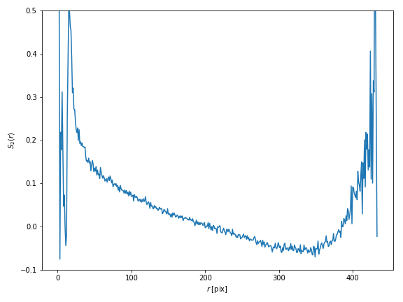
For small values of $r$, the curve is not relevant, since very little grains are close enough (remember that rice grains are non-overlapping particles!). Similarly, the increase at large values of the center-to-center distance $r$ should be considered with caution. Indeed, due to the limited size of the specimen, sampling is insufficient at high $r$. For intermediate values of $r$, the curve is interesting. It shows a rather good correlation at small distances, but this correlation decreases rapidly. For larger values of $r$, we do not observe $S_2(r)\to0$, which might reflect the fact that the specimen is not isotropic (as shown in the previous section); this should be investigated further.
Boundary effects
To close this post on orientation correlations, we investigate boundary effects in the specimen. The wall of the cylindrical sample container is impenetrable. Therefore, the particles closest to the wall are tangent this wall. We want to quantify the distance over which the grains keep the memory of this preferred orientation.
To do so, for each grain, we locate the closest point on the wall, and the corresponding normal vector. We first recall the location of the axis of the container, and its radius (see this post).
x_center = 219
y_center = 217
radius = 208
We then compute the radius-vector (we discard the $z$-coordinate, which is the first index), from which we deduce the normal to the boundary, $\vec e_r$.
radius_vector = center-[0, x_center, y_center]
# Discard first (z) coordinate!
distance_to_axis = np.sqrt(np.sum(radius_vector[:, 1:]**2, axis=-1))
distance_to_boundary = radius-distance_to_axis
e_r = radius_vector/distance_to_axis[:, None]
e_r[:, 0] = 0
We now compute the orthoradial vector $\vec e_\theta$,
e_theta = np.zeros_like(e_r)
e_theta[:, 1] = -e_r[:, 2]
e_theta[:, 2] = e_r[:, 1]
For each grain, the direction $\vec n_i$ is decomposed in the local basis $(\vec e_r, \vec e_\theta, \vec e_z)$.
orientation_local = np.zeros_like(orientation)
orientation_local[:, 0] = np.sum(e_r*orientation, axis=-1)
orientation_local[:, 1] = np.sum(e_theta*orientation, axis=-1)
orientation_local[:, 2] = orientation[:, 0]
We then compute the matrix representation of the tensor $\vec n_i\otimes\vec n_i$ in the local basis.
nxn = orientation_local[:, :, None]*orientation_local[:, None, :]
labels = np.round(distance_to_boundary/4)*4
indices = np.unique(labels)
nxn_mean = np.array([[scipy.ndimage.mean(nxn[:, i, j], labels, indices)
                      for j in range(3)] for i in range(3)])
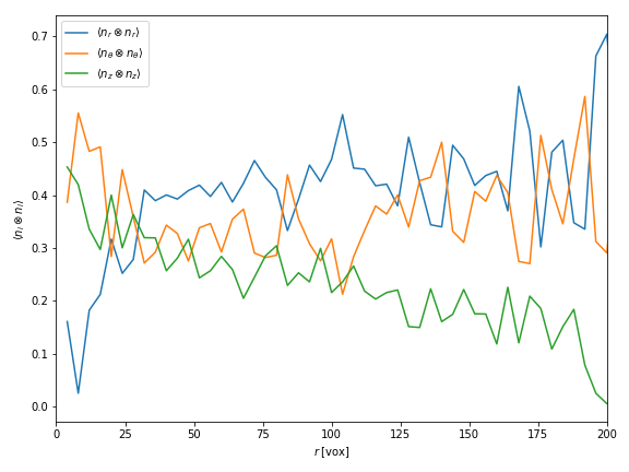
The resulting statistical descriptors are plotted in Fig. 2. Honestly, the results are not very conclusive. Both $\langle n_r\otimes n_r\rangle$ and $\langle n_\theta\otimes n_\theta\rangle$ seem to decrease rapidly over a distance of (roughly) 30 voxels. However, they both converge to a value which is non-zero.
fig = mpl.figure.Figure(figsize=(8, 6))
ax = fig.add_subplot(1, 1, 1)
ax.set_xlabel(r'$r\;[\mathrm{vox}]$')
ax.set_ylabel(r'$\langle n_i\otimes n_i\rangle$')
ax.set_xlim(0, 200)

ax.plot(indices, nxn_mean[0, 0],
        label=r'$\langle n_r\otimes n_r\rangle$')
ax.plot(indices, nxn_mean[1, 1],
        label=r'$\langle n_\theta\otimes n_\theta\rangle$')
ax.plot(indices, nxn_mean[2, 2],
        label=r'$\langle n_z\otimes n_z\rangle$')
ax.legend(loc='upper left')

fig.tight_layout()
fig.savefig('boundary_effects.png', transparent=True)
/usr/lib/python3/dist-packages/matplotlib/tight_layout.py:231: UserWarning: tight_layout : falling back to Agg renderer
  warnings.warn("tight_layout : falling back to Agg renderer")
Conclusion
This was the last post of this series on Orientation correlations among rice grains. This post was dedicated to the quantification of orientation correlations. To do so, we have recalled the definition of several statistical descriptors. These descriptors were then evaluated on the sample.
The resulting values indeed indicate the existence of orientation correlations. However, further investigations should be carried out in order to draw reliable conclusions. In particular, the descriptors plotted in Figs. 1 and 2 are histograms, and filtering of some sort should be used to smooth the curves. Besides, the analysis of the first section shows that the sample is globally anisotropic. This global anisotropy should be accounted for (“subtracted”) while analyzing local anisotropy. In short, the present post should be considered as a mere introduction to the matter and the relevant tools.
Well, I hope you enjoyed this series! We initially set out to quantify orientation correlations in an assembly of rice grains. To do so, a fair amount of image analysis was required. We introduced binning, the Hough transform, Otsu's method, a dedicated seeding technique for the watershed transform and the quantification of the morphology of the grains. All these techniques have a wide range of applications, which goes far beyond the analysis of rice grains!