On the periodic-plus-smooth decomposition of an image, part 5: minimizing the energy, the clumsy way

In this post, we will compute Moisan's (2011) periodic-plus-smooth decomposition of an image by direct minimization of the energy introduced in the second instalment of this series. More precisely, $u$ being a $m\times n$ image, we will minimize the function $F(v, u)$ over the space of $m\times n$ images $v$. The minimizer, $s$, is the smooth component of $u$, while its complement $p=u-s$ is the periodic component of $u$. This post is the fifth instalment of a series in seven parts:

1. Introduction
2. Defining the decomposition
3. The energy as a quadratic form
4. Implementing the linear operators
5. Minimizing the energy, the clumsy way
6. Minimizing the energy, the clever way
7. Improved implementation of Moisan's algorithm

The code discussed in this series is available as a Python module on GitHub.

We showed in part 3 that $F$ was in fact a quadratic form, and expressed the underlying linear operators, which were subsequently implemented in part 4. It is recalled (see part 3) that

$$F(v, u)=\langle v, Q\cdot v\rangle-2\langle v, Q_1\cdot u\rangle+\langle u, Q_1\cdot u\rangle,$$

where $Q$ and $Q_1$ are symmetric, positive linear operators. Minimizing $F$ with respect to $v$ therefore amounts to solving the linear system: $Q\cdot s=Q_1\cdot u$. It can in fact be shown that $Q$ is positive definite, therefore the solution to this linear system is unique: $s=Q^{-1}\cdot Q_1\cdot u$. It can be computed by means of the conjugate gradient method, as illustrated below.

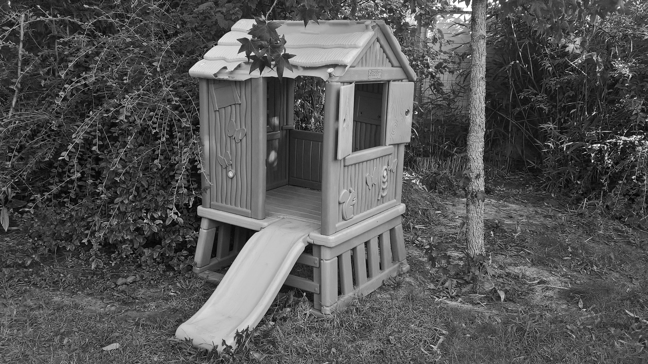
Let us start by loading up some modules and the input image to be periodized (see Fig. 1).

import numpy as np

from scipy.sparse.linalg import cg
from skimage.io import imread, imsave

u = imread(DATA_DIR+'hut-648x364.png')
u = u.astype(np.float64)

We then create the operators $Q_1$ and $Q$ that were implemented in the previous instalment of this series.

Q1 = OperatorQ1(u.shape)
Q = OperatorQ(u.shape)

We then compute the right-hand side of the system, namely $Q_1\cdot u$. Attention must be paid to the fact that $u$ must be flattened to a 1D array.

m, n = u.shape
Q1u = Q1@u.reshape((m*n,))

We then use the scipy.sparse.linalg.cg function (see documentation) to solve the linear system

x, info = cg(Q, Q1u)
if info == 0:
    print('success!')
else:
    print(info)
s = x.reshape(u.shape)
p = u-s

We can now save the results (for future reference).

def to_uint8(v):
    m, n = v.shape
    v_min = v.min()
    v_max = v.max()
    return (255.0*(v-v_min)/(v_max-v_min)).astype(np.uint8)

imsave(DATA_DIR+'hut-648x364-smooth-cg.png', to_uint8(s))
imsave(DATA_DIR+'hut-648x364-periodic-cg.png', to_uint8(p))
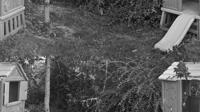
imsave(DATA_DIR+'hut-648x364-periodic-cg-fftshift.png',
       to_uint8(np.fft.fftshift(p)))

Again, periodization is best observed by swapping the quadrants (see Fig. 2).

Et voilà…

In this fairly quick post, we derived a reference periodic-plus-smooth decomposition of a specific image. The conjugate gradient iterations are highly inefficient, and we will show in the next instalment of this series that a very efficient alternative, based on the fast Fourier transform, was proposed by Moisan (2011). The decomposition that we obtained in the present post will then be used as a reference for testing our implementation of Moisan's algorithm.