In the previous instalment of this series, we computed Moisan's (2011) periodic-plus-smooth decomposition of an image by means of the conjugate gradient method. This worked like a charm, but was fairly inefficient, owing to the iterative nature of the method. Moisan actually showed that the whole decomposition could be computed explicitly in Fourier space. This will be discussed in the present post, which is the sixth in a series in seven parts:
- Introduction
- Defining the decomposition
- The energy as a quadratic form
- Implementing the linear operators
- Minimizing the energy, the clumsy way
- Minimizing the energy, the clever way
- Improved implementation of Moisan's algorithm
The code discussed in this series is available as a Python module on GitHub.
Before we proceed, let us recall how the discrete Fourier transform $\hat{u}$ of the $m\times n$ image $u$ is defined
$$\hat{u}_{\alpha\beta}=\sum_{i=0}^{m-1}\sum_{j=0}^{n-1}u_{ij}\exp\Bigl[-2\pi\mathrm i\Bigl(\frac{\alpha i}m+\frac{\beta j}n\Bigr)\Bigr],$$
for $\alpha=0, \ldots, m-1$ and $\beta=0, \ldots, n-1$. We have the well-known inversion formula
$$u_{ij}=\frac1{mn}\sum_{\alpha=0}^{m-1}\sum_{\beta=0}^{n-1}\hat{u}_{\alpha\beta}\exp\Bigl[2\pi\mathrm i\Bigl(\frac{\alpha i}m+\frac{\beta j}n\Bigr)\Bigr].$$
The remainder of this post is organized as follows. We will first introduce Moisan's algorithm (2011). Then a first implementation of this algorithm will be proposed and tested. Improved implementations will be discussed in the next instalment of this series.
Moisan's algorithm
It is recalled (see previous post) that the smooth component $s$ of a $m\times n$ image $u$ is found from the solution to the following linear system
$$Q\cdot s=Q_1\cdot u,\tag{1}$$
where $Q$ and $Q_1$ are symmetric, positive linear operators defined in part 3 of this series ($Q$ is actually positive definite). As observed in part 4 of this series, operator $Q$ is in fact the sum of the periodic convolution operator with the following kernel
$$\begin{bmatrix} 0 & -2 & 0\\ -2 & 8 & -2\\ 0 & -2 & 0 \end{bmatrix}$$
and the operator that maps any image $u$ onto the constant image equal to $\operatorname{mean}u/mn$. It then results from the circular convolution theorem that
$$(\widehat{Q\cdot s})_{\alpha\beta}=\left\{\begin{array}{ll}m^{-2}n^{-2}\hat{s}_{00} & \text{if }(\alpha, \beta) = (0, 0),\\ \bigl(8-4\cos\frac{2\pi\alpha}m-4\cos\frac{2\pi\beta}n\bigr)\hat{s}_{\alpha\beta} & \text{otherwise}.\end{array}\right.\tag{2}$$
Combining Eqs. (1) and (2), we find the following expression of the discrete Fourier transform of the smooth component $s$
$$\hat{s}_{\alpha\beta}=\frac{\hat{v}_{\alpha\beta}}{2\cos\frac{2\pi\alpha}m+2\cos\frac{2\pi\beta}n-4}\quad\text{for}\quad(\alpha, \beta)\neq(0, 0),\tag{3}$$
where we have introduced $v=-\frac12Q_1\cdot u$. Since $\operatorname{mean}s=0$, we also have $\hat{s}_{00}=0$. From the definition of $Q_1$ (see part 3 of this series), we have $v=v^\mathrm h+v^\mathrm v$, with
$$v^\mathrm h_{ij}= \left\{ \begin{array}{ll} u_{i, n-1}-u_{i, 0} & \text{if }j=0,\\ u_{i, 0}-u_{i, n-1} & \text{if }j=n-1,\\ 0 & \text{otherwise}, \end{array}\right.\tag{4a}$$
and $$v^\mathrm v_{ij}= \left\{ \begin{array}{ll} u_{m-1, j}-u_{0, j} & \text{if }i=0,\\ u_{0, j}-u_{m-1, j} & \text{if }i=m-1,\\ 0 & \text{otherwise}. \end{array} \right. \tag{4b}$$
Moisan's algorithm (2011) readily follows from this analysis
- compute $v$ [use Eq. (4)],
- compute its discrete Fourier transform $\hat{v}$,
- compute $\hat{s}$ [use Eq. (3)],
- compute its inverse discrete Fourier transform $s$,
- compute $p=u-s$.
Of course, the fast Fourier transform will be used for steps 2 and 4.
A first implementation of Moisan's algorithm
Reference implementation of Moisan's algorithm results directly from the above analysis.
def _per(u, inverse_dft=True):
    """Compute the periodic component of the 2D image u.

    This function returns the periodic-plus-smooth decomposition of
    the 2D array-like u.

    If inverse_dft is True, then the pair (p, s) is returned
    (p: periodic component; s: smooth component).

    If inverse_dft is False, then the pair

        (numpy.fft.fft2(p), numpy.fft.fft2(s))

    is returned.

    This is a reference (unoptimized) implementation of Algorithm 1.
    """
    u = np.asarray(u, dtype=np.float64)

    v = np.zeros_like(u)
    du = u[-1, :]-u[0, :]
    v[0, :] = du
    v[-1, :] = -du

    du = u[:, -1]-u[:, 0]
    v[:, 0] += du
    v[:, -1] -= du

    v_dft = np.fft.fft2(v)

    m, n = u.shape
    cos_m = np.cos(2.*np.pi*np.fft.fftfreq(m, 1.))
    cos_n = np.cos(2.*np.pi*np.fft.fftfreq(n, 1.))

    k_dft = 2.0*(cos_m[:, None]+cos_n[None, :]-2.0)
    k_dft[0, 0] = 1.0
    s_dft = v_dft/k_dft
    s_dft[0, 0] = 0.0

    if inverse_dft:
        s = np.fft.ifft2(s_dft)
        return u-s, s
    else:
        u_dft = np.fft.fft2(u)
        return u_dft-s_dft, s_dft
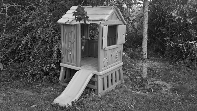
Which can be applied to the following image.
import numpy as np

from skimage.io import imread, imsave

u = imread(DATA_DIR+'hut-648x364.png')
u = u.astype(np.float64)
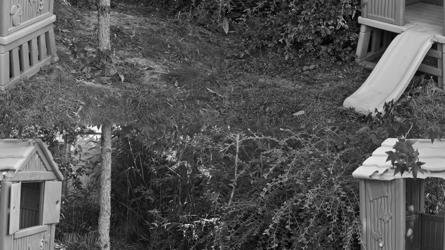
The periodic-plus-smooth decomposition is then computed as follows.
p, s = _per(u, inverse_dft=True)

imsave(DATA_DIR+'hut-648x364-periodic-_per-fftshift.png',
       np.fft.fftshift(p.real).astype(np.uint8))
Which results in the following image ($p$ has been FFT-shifted, in order to demonstrate the effect of periodization).
It should be noted that the resulting decomposition is a pair of complex images (since we used the complex DFT to perform the decomposition). We ought to check that the imaginary parts of $p$ and $s$ are indeed nearly null
print('Imaginary part of')
print('  p: min = {}, max = {}'.format(p.imag.min(), p.imag.max()))
print('  s: min = {}, max = {}'.format(s.imag.min(), s.imag.max()))
Imaginary part of
  p: min = -2.6931883320843306e-12, max = 4.161745834921434e-12
  s: min = -4.161745834921434e-12, max = 2.6931883320843306e-12
We can then readily set $p$ and $s$ to their real parts
p_act = p.real
s_act = s.real
Testing our implementation
In the previous instalment of this series, we computed a reference periodic-plus-smooth decomposition by means of the conjugate gradient method. Let's do that again.
from scipy.sparse.linalg import cg

tol = 1E-8
Q1 = OperatorQ1(u.shape)
Q = OperatorQ(u.shape)
m, n = u.shape
b = Q1@u.reshape((m*n,))
x_exp, info = cg(Q, b, tol=tol)
if info == 0:
    res_exp = np.linalg.norm(b-Q@x_exp)
    print('Residual: {}'.format(res_exp))
else:
    print(info)
s_exp = x_exp.reshape(u.shape)
p_exp = u-s_exp
Residual: 3.9422689362828e-05
We can then compute the norm of the difference
abs_err = np.linalg.norm(s_act-s_exp)
rel_err = abs_err/np.linalg.norm(0.5*(s_act+s_exp))
print('Error in L2-norm:')
print('  - absolute: {}'.format(abs_err))
print('  - relative: {}'.format(rel_err))
Error in L2-norm:
  - absolute: 0.004504952971826568
  - relative: 1.3139651711483983e-06
This is already quite satisfactory. We can also compute the residual with the value of $s$ found through the DFT approach
x_act = s_act.reshape((m*n,))
res_act = np.linalg.norm(b-Q@x_act)
print('Residual: {}'.format(res_act))
Residual: 1.8964547594731774e-11
Which is much smaller than the residual obtained through conjugate gradient iterations! Surely, our implementation delivers the correct periodic-plus-smooth decomposition!
Conclusion
In the present post, we have implemented Moisans's algorithm (2011) for computing the periodic-plus-smooth decomposition of an image. This algorithm is much faster than our previous implementation, relying on the conjugate gradient method. We will show in the next instalment of this series that we can do slightly better, though.